Data
Juan Orduz
Oct 20, 2023
Using Causal Inference for Offline Campaign Analysis Measurement

This blog post summarizes our Data Scientist Juan Orduz’s talk from our Data Science meetup. You can watch the full talk below or jump into the recap of the talk highlighting the main techniques for using causal inference techniques to measure offline marketing campaign performance. Happy reading and watching!
Recap of the talk:
Traditionally, offline channels like TV and out-of-home advertising (such as billboards) have been critical channels in the marketing mix to drive brand awareness and direct sales. But how can we measure their efficiency? In his talk, Juan worked out a simulated example to illustrate how the marketing tech data science team at Wolt uses causal inference techniques to measure offline marketing campaign performance. The motivation for these measurements is clear: we need to understand media efficiency to optimize it. The work on experimentation is a key component of our holistic measurement system at Wolt which consists of two main pillars: attribution and media mix models. Let’s explore this more in a simulated example.
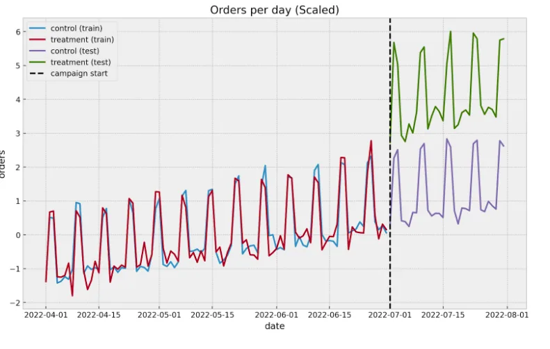
We have found that a great strategy to illustrate and test analytical techniques is to work out a simulated example. This way, you can test the results against true quantities, which you don’t have in real-life cases. To illustrate some of the methodologies, we’re going to simulate an offline campaign across a given geo, say a city or a country region. For this specific campaign, we can buy media at the zip code level. Each zip code was assigned to a variant: treatment and control. We assume the zip codes belong to different districts to avoid spillover effects (even though, in real life, this is a problem by itself). Still, the districts are “comparable” (details on this below) The treatment can be something like an out-of-home campaign (billboards) or flyers. In this simulated example, we fully control the treatment effect to test various methodologies. Here’s what the data looks like:
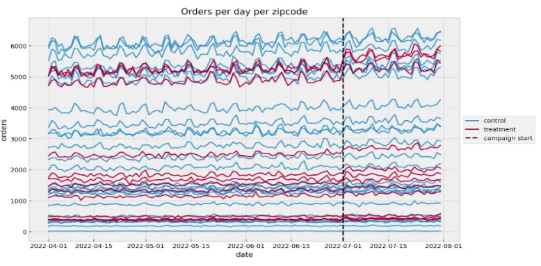
The figure above shows the time series development of orders across zip codes split by variant (control = no campaign, treatment = campaign). There are two things we immediately see as common characteristics of these time series:
All of them have a positive trend component — this means that overall orders are increasing over time for both variants
There’s a clear weekly seasonality component — note that orders usually increase during the weekends
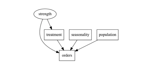
This is, of course, intentionally added to the data generation process. In addition, we include an unobserved feature, “strength,” which represents the brand presence at the zip code level (a district-dependent feature) and which we assume doesn’t change over time for simplicity. We added this feature as, in real cases, we have many unobserved confounders we need to deal with.
During the talk, we went through various approaches subjected to data availability. Let’s have a brief look at each case.
Case 1: No control group
Sometimes it takes work to set up a proper control group. So let’s start with such a case. A naïve approach would be to compare the orders pre- and post-campaign simply as:
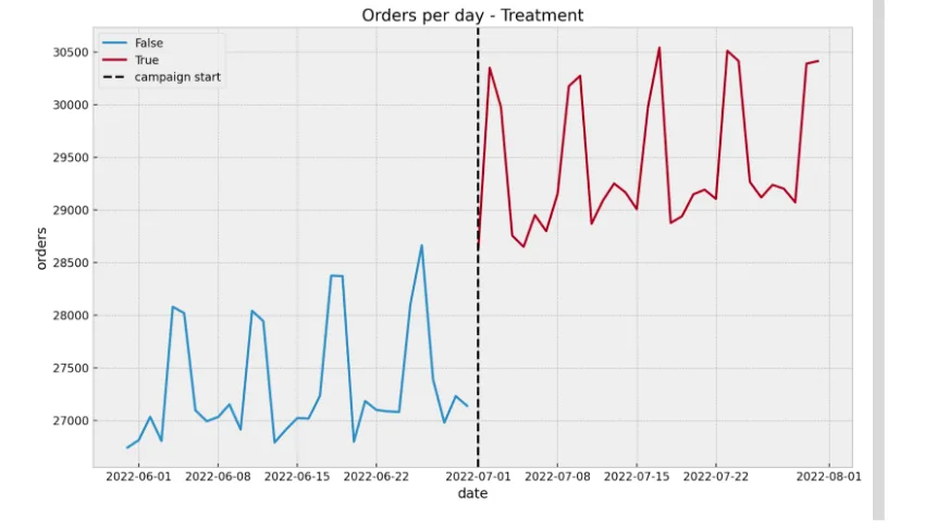
This simple approach will overestimate the campaign's effect as we’ll attribute the trend and seasonality contributions. Note that organically we have orders growing over time. How can we get a better estimate? Observe that the fundamental problem is that there’s no way to deterministically know how the orders would’ve developed had there been no campaign. Often people refer to this as the counterfactual. This is the core problem of causal inference. All the methods described in this talk and blog post aim to estimate such counterfactuals through different techniques.
A first natural strategy is to use time series forecasting methods. A common approach is to use a Bayesian structural time series model as in Google’s CausalImpact package. The benefit of this approach is that the time series model will lead the trend and seasonal components from historical data and encode this into the counterfactual (solving the main problem of the naïve approach). We fit such a model on the aggregation of the campaign zip codes. The following plot summarizes the results of the model. The upper plot shows the true and predicted values (counterfactual) of the time series model. Note that these predictions capture the linear growth and the weekly seasonality. The middle plot is the pointwise difference between the true and predicted values. The lower plot shows the cumulative difference. From this last plot, we see that based on the model predictions, we estimate 50K orders coming from the offline campaign. In practice, we’d add a cool-down period to allow for delayed effects, but we omit this for simplicity.
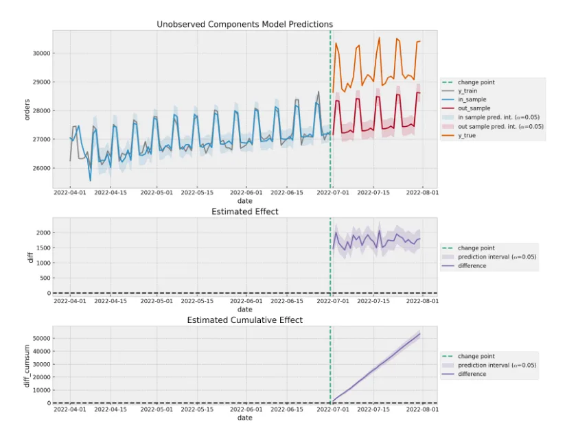
When using these techniques, it’s essential to quantify the model and effect estimation uncertainty, as you want to avoid allowing noise from the training step to be attributed to the campaign effect. Methods like time-slice-cross validation should be part of the analysis.
Case 2: We have control groups and a linear relation
In this case, we want to use the control group to use a simpler method (not a Bayesian structural time series model, for example) to control for the trend and seasonality components.
One common approach is a time-based regression where we assume (we can test this hypothesis) that there’s a linear relationship between the aggregated orders between the control and treatment zip codes. Under this assumption, we can use a linear regression model to estimate the counterfactual. The marketing tech team at Wolt has a strong affinity for Bayesian methods (this framework allows us to build complex custom models where we can pass business constraints via priors). Hence, we use Bayesian linear regression to quantify the uncertainty better. The following plot shows the (scaled) aggregates of the treatment and control groups. Before the campaign starts, there’s indeed a linear relationship between the two groups.
After running the regression model and scaling the cumulative effect, the results are comparable with the CausalImpact approach above because our simulated data is dominated by the positive trend and seasonality, which are encoded in the aggregation of the control group time series. In general, having a control group improves the variance of the estimation and makes the result much more interpretable.
Case 3: We have control groups, but no linear relation necessarily
Synthetic Control
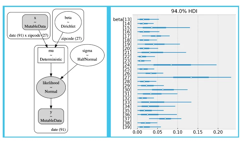
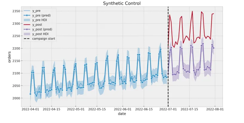
Requiring linearity is often a strong requirement. In cases where the linearity doesn’t hold, we can create a synthetic control by considering a convex combination of the control zip codes. That means we run a linear regression with control zip codes as control where we enforce the coefficient to be positive and add up to one. These constraints are helpful to avoid overfitting when generating the synthetic control as we enforce the control units to interpolate instead of extrapolate. The following plot shows the model specification and coefficients for the synthetic control.
Once the model is fitted, we can estimate the counterfactual:
Fixed Effects Model
There are many other methods to estimate campaign effectiveness when we have a control group, for example, difference-in-difference. One method we have used in practice and has proven very successful is panel data and fixed effect models. The idea is not to aggregate the data but use individual zip code data to estimate a global effect. We do so by cleverly controlling the zip code and time (think about dummy variables).
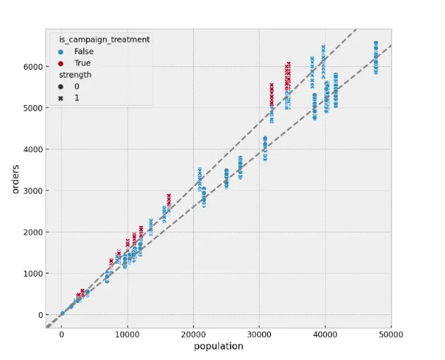
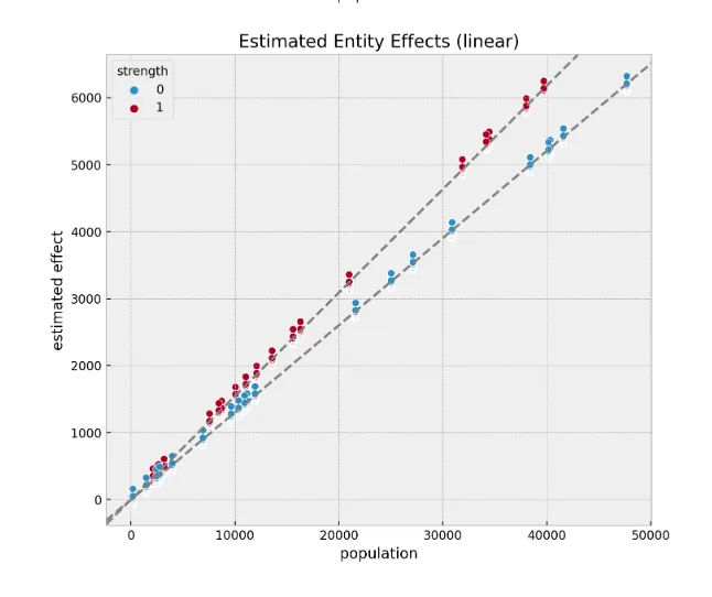
One of the greatest benefits of this approach is that it takes care of the unobserved confounders, which are invariant over time, like our strength feature above. The following two plots show this. The left one shows the orders as a function of the population using the synthetic data where we have the strength feature (which we generally would not observe). Notice there are two linear components with different slopes. They correspond to the two levels of strength. On the right-hand side, you see the results from the fixed effect models. Although we don’t measure the feature strength, the model was able to factor it out as part of the treatment effect estimation!
Conclusion
In this blog post, we used a synthetic data set to illustrate various techniques to estimate the direct effects of offline marketing campaigns. Concretely, we looked into Bayesian structural time series models (causal impact), time-based regression, synthetic control, and panel data methods. But it’s good to note that ultimately there’s no silver bullet to solve all problems when measuring offline marketing campaign effectiveness. It depends on the exact data and the business problem being solved!
As an essential remark, these techniques are insufficient to provide the whole picture of the marketing funnel. For example, TV campaigns can have a significant delayed effect through brand awareness. We aim to evaluate channel (and channel mix) performance holistically through the combination of attribution models, media mix modeling, and experimentation. For these later cases, all the causal inference techniques described in this post are an essential part of the analyst toolbox.
References:
Inferring Causal Impact Using Bayesian Structural Time-Series Models
Estimating Ad Effectiveness Using Geo Experiments in a Time-Based Regression Framework
Hungry for more details on the topic? Watch Juan's full talk below 👇